Craig Coker
This series on odor management, available in the BioCycle archives (www.biocycle.net), has covered how and where odors are generated, measured, and perceived; how they are managed through good process control; how they are controlled with technology; how to manage the public outreach related to organics recycling odors; and the basics of atmospheric dispersion.
No matter how well planned, sited or managed, composting facilities are always at risk for an off-site odor episode that can create challenges such as negative publicity, regulatory intervention and lawsuits. This article series has been dedicated to helping composters understand the intricacies of odor management. Part VII looks at the topic of odor modeling and the challenges of mathematically simulating a dynamic environment.
Simulation of the movement of environmental pollutants in the natural world using computer tools is always challenging. Models have to simulate the real-world dynamics where environmental conditions can change in three dimensions (length, breadth and height) and also in time. Numerical simulations solve simultaneous equations at discrete points in 3-dimensional space, known as a grid or mesh. Calculations at each grid point have to be averaged over some time period to account for temporal changes. For environmental pollutants that can change their characteristics (such as the conversion of sulfur dioxide (SO2) to sulfur trioxide (SO3) by sunlight), those chemical changes also have to be interpreted by the equations in the models. These are among the computational aspects that make odor modeling so challenging and difficult.
Odor modeling is an outgrowth of the air pollutant dispersion modeling used to predict distant concentrations of criteria air pollutants from continuous point sources, like smokestacks, or from continuous line sources, like highways. These models allow for the determination of compliance with a criteria air pollution standard, such as the 0.5 parts per million (ppm) limit for a 3-hour average value of SO2. Passage of the Emergency Planning and Community Right-to-Know Act in 1986 furthered development of air pollution dispersion models that could simulate a “one-time” release of air pollutants into the environment; these models were derived from volcanic ash emission models.

Figure 1. Gaussian dispersion plume
The oldest and most widely used models are known as Gaussian dispersion models, which assume pollutant dispersion is more a function of wind turbulence than vertical (temperature) turbulence. This model assumes that the average (hourly) concentration of a contaminant downwind of a source and perpendicular to the average wind direction is normally distributed and centered along the wind direction from that source (Figure 1). These models are most often used for predicting dispersion of continuant, buoyant plumes originating from ground level or elevated sources.
Some odorous plumes are buoyant; others are not. A plume is buoyant if it is warmer than ambient air, or if the pollutant has a lower molecular weight than air. Most odorous plumes rising from composting facilities are heated, so they tend to rise, then sink as they cool off.
Input required for Gaussian dispersion models includes meteorological data, the concentration or quantity and temperature of the pollutant source, emissions parameters, terrain elevations and dimensions of obstructions. Meteorological data inputs are wind speed and direction, amount of atmospheric turbulence (as characterized by the stability class), ambient air temperature, inversion height, cloud cover and solar radiation. Emissions parameter inputs are source location and height, type of source, and exit velocity and mass flow rate of the plume. Terrain data includes ground elevations at the source and at the locations of any sensitive receptors. Obstructions include buildings or other structures that may interrupt the plume flow path, so the dimensions of those obstructions are needed. The old computer adage of “garbage in, garbage out” applies to dispersion modeling. Accurate modeling results require that local meteorological data is used and that the other data inputs are precisely measured.
")
Figure 2. Odor dispersion model (odor units/m3) Source: OdoWatch/OdoTech
Output is usually a map of the modeled concentrations of the pollutant in question over the area modeled. These are often drawn as lines of equal concentration (known as “isopleths”) that resemble the elevation lines on a topographic map. This mapping concept spatially relates dispersion of the concentration of an air pollutant at a source to the concentration at the receptor’s location. This concept is illustrated in Figure 2.
Measuring Odor Concentration
Odor modeling is not as definitive as single-pollutant conventional air dispersion models. One odor “flavor wheel” in use lists 53 different odorous chemicals. As odors are made up of multiple chemicals, modeling becomes more difficult. Because of this multitude of odorous gases, odor modeling uses a surrogate measure of concentration. Models can be set up with the source emissions characterized in terms of dilution-to-threshold (D/T) at a source inside the composting facility where the odors are strongest, as determined by an odor panel. D/T represents a dilution factor, measured by the number of volumes of odor-free air needed to dilute odorous air to the point where 50 percent of an odor panel cannot detect the odor. The source emission rate could therefore be 50 D/T, which is modeled to be a D/T of 2 at a certain distance. As D/T is dimensionless, sometimes an artificially derived measure of odor units per cubic meter (OU/m3) is used to create the impression that an actual odor concentration is being modeled.
“These types of odor models are essentially a risk management strategy,” says Ray Porter, Knowledge Leader at Odotech, an odor monitoring and modeling consultancy headquartered in Montreal, Quebec, Canada. “Models overlay multiple worst-case scenarios in meteorology and odor emissions and predict the threat of an odor impact at levels of risk that relate to detection and recognition thresholds for odors. Modeling for odor exposure at the detection threshold is one level of risk; modeling for the recognition threshold represents a higher level of risk. The question is: ‘What is the likelihood that this receptor will experience an adverse odor impact?’” Porter adds it is important to quantify the initial odor emissions estimate based on source data determined by an odor panel made up of representatives of the public.
Odor dispersion modeling is also sensitive to the time averaging period of the model. Most dispersion models were developed to predict compliance with the National Ambient Air Quality Standards, which define acceptable pollutant concentrations in ambient air averaged over exposure times of 1 to 24 hours. These models predict the concentration of a pollutant that would be present in a mixed sample of ambient air that had been sampled over a 1-hour period. Averaging over a specified period smoothes out some of the variations in the air pollutant concentration, concealing peaks that may result from short-term variations in emission rates and in meteorological conditions.
Averaging Impacts
Odors are much more transient, varying in concentration and intensity in a matter of minutes, so air models with one-hour averaging times cannot accurately represent the short-term nature of odors. Adjustments must be made to use shorter averaging times. Peak-to-mean ratios are used to adjust model averaging times. In selecting an averaging period for an odor impact assessment, consideration must be given to the limits of such an analysis. A person might be able to detect an odor in 1 to 3 seconds, but it is more likely that a period of 3 to 5 minutes of exposure to the odor is needed to invoke an odor complaint, so 5 minutes averaging time is often used in odor modeling. Averaging times can be adjusted using a Power Law relationship, which is defined as follows:
C1 = C0 * ( t0 / t1 ) p
where:C0 = the initial (1-hour average) concentration
C1 = the concentration at the desired averaging period
t0 = the initial (60-minute) averaging period
t1= the desired averaging period (minutes)
p = power law exponent (varies from 0.17 to 0.68)
The power law relates the peak-to-mean concentration ratio (C1, C0) to the short-to-large term average time ratio (t0, t1). This relationship was found to provide a reasonable approximation of peak-to-mean ratios across all stability categories (Porter, 2012).
This equation was used to adjust predicted concentrations of “odor units” in an odor modeling study at a composting facility in Lisbon, Portugal (Riberio, 2010). Odor emission rates varied from 430 to 3,200 OU/m3 at the facility, as determined by an odor panel. The regulatory standard modeled was the German standard of less than 10 percent “odor hours” per year in residential areas and less than 15 percent in industrial areas. German regulations define an “odor hour” as an hour in which there is a clear odor perception for at least 10 percent of the time. The analysts used the EPA’s Industrial Source Complex Short-Term (ISCST3) dispersion model, which is widely used in conventional air pollutant modeling. They used the Power Law equation above to adjust the averaging period to 5 minutes and modeled the odor emissions on a 250 meter (m) by 250 m grid. This finer-grained level of analysis allowed them to determine that an area up to 1,500 m south of the facility would likely fail to meet the German 10 percent odor-hour standard.
Detailed quantitative analysis is possible with dispersion models adjusted to shorter time averaging periods. These models predict a numerical “dilution” at the receptor, but what is an acceptable level of probability that the predicted number (D/T or OU/m3) will be exceeded? “It is possible to model noise impacts against a standard of maximum acceptable noise level,” observes Thierry Page, CEO of Odotech, “but with odors, we’re dealing with perception of nuisance. In the real world of odors, perception induces interpretation and speculation. These models, even if imperfect, are still useful, provided they are constructed by reference methods.” In the U.S., the primary reference method used is ASTM Standard of Practice E679-91, “Determination of Odor and Taste Threshold by a Forced-Choice Ascending Concentration Series Method of Limits,” which is the reference method for the odor panel determination of initial odor concentration to be modeled mentioned above.
Other methods of modeling odors are to use Lagrangian “puff” models or computational fluid dynamics (CFD). Lagrangian models mathematically follow pollution plume parcels as they move in the atmosphere (it is said that an observer of a Lagrangian model follows along with the plume). One model in widespread use is CALPUFF, which is designed to simulate continuous puffs of pollutants emitted from a source into the ambient wind flow. As the wind changes, the path each puff takes follows a new wind direction. Diffusion of the puffs into the air is calculated as a Gaussian distribution and pollutant concentration at or near a receptor and is based on the contribution of each puff as it passes by. CALPUFF has been used to model odor dispersion from livestock operations, with agreements between model predictions and measured odor intensities ranging from 37 percent to 50 percent (Li, 2006).
CFD numerically solves the basic governing equations of mass, momentum and energy within each cell in a three-dimensional Cartesian grid. The method uses a Eulerian-Lagrangian approach to simulate atmospheric dispersion (it is said that an observer of a Eulerian model watches the plume go by). In an evaluation of odors from a 3,000-sow farrowing operation in Canada, the Eulerian-Lagrangian approach used trajectories of discrete “odor gas parcels” to predict the dispersion of odorants. The governing equations in CFD modeling are the Navier-Stokes equations, which describe the motion of fluid substances in terms of the conservation of mass, momentum and energy. These equations are applied to airflow as a fluid, modeling, for example, airflow around an airplane wing.
CFD can be used for extremely fine-grained analysis or for larger-scale odor and dust studies. “CFD models used to be run on large mainframe computers, but with the improvements in desktop PCs, CFD models can be run by mere mortals like me,” says Ray Kapahi, Principal with Air Permitting Specialists based in Sacramento, California. Kapahi’s firm recently used CFD to model dust emitted from bulk stockpiles of sand at a landscape supply yard near Stockton, California in response to neighbors’ complaints of dust leaving the supply yard site.
“While we were doing a 2-dimensional dust study, we would use this same approach for doing an odor study,” notes Kapahi. “We modeled the site by digitizing all the buildings on–site into the model from a Google Maps image, assumed a dust source emissions rate of 0.1 kg/sec, assumed a wind speed of 0.1 m/sec, and used a 500 m by 500 m grid with 1-m grid spacing.” An illustration from the dust model output is shown in Figure 3. Kapahi adds that when modeling odors, it is possible to use CFD to model in three-dimensional space, thus allowing for the model to account for vertical dispersion in the atmosphere due to turbulent mixing. With grid spacing as close as 1 cm by 1 cm and a time scale of 5-second intervals, it would be possible to model odor emissions at each of the houses in a neighborhood downwind of a composting facility.
CFD was used to model odor emissions from a 3,000-head hog operation in southern Manitoba, Canada (Li, 2006). The CFD model’s 3-dimensional approach used trajectories of discrete “odor gas parcels” (OGPs) to predict dispersion of odorants. In this study, the investigators set up a modeling domain of a 5,000 m radius and 200 m tall cylinder over the farm, with a total of 200,000 computational cells in the modeling domain. The model assumed OGPs were emitted continuously, had a size of 1 x 10⁻⁶ m diameter, and had an initial emission rate of 191,923 OU/second. The model predicted odor concentration at 1.5 m height within 5,000 m after one hour. An odor standard of 2 OU/m3 was used as a compliance boundary and the model computed that the odor travel distance for achieving 2 OU/m3 was 860 m under unstable atmospheric conditions and 5,610 m under the most stable conditions.
A number of analytical computational tools can be used to model odor emissions and predict impacts on nearby (and distant) receptors. All modeling tools are risk management approaches, essentially predicting the number of occurrences in a given time period when a predicted odor level will occur. If odor standards were quantitative standards, like air pollution standards, then modeling would be an essential tool for composting facility siting, design and management. The reality is, though, that odor standards are subjective nuisance standards and there is lack of agreement among composters, elected and staff officials, and the general public as to what is an acceptable level of inconvenience.
Craig Coker is a Contributing Editor to BioCycle and a Principal in the firm Coker Composting & Consulting (www.cokercompost.com), near Roanoke VA. He can be reached at cscoker@verizon.net.